Creating generative art using flow fields
Up to this point in my life, I've never before had a big interest in making or "participating" in graphical art. My creativity and artistic inclinations have always been more musical, including making hip-hop beats using FLStudio and playing guitar with friends.
I recently came across some artwork created by Tyler Hobbs, who is an artist that has a focus on generative works. His creations include generating lines and shapes within a flow field, which result in highly rich, textured, and unique artworks. It's the kind of art that would just look fantastic hanging up prominently in the living room for all to enjoy!
I loved his Fidenza series in particular and felt deeply moved and inspired. I felt a desire to try my hand at creating similar artworks – below, I walk through that process, including what I learned from Tyler's articles on how to achieve these styles and patterns using flow fields and the code that I wrote to get these results.
How to draw with code
For this project, I wanted to use Python for its easiness and support for the libraries that would make this endeavor much simpler. Case in point, the Turtle library comes out-of-the-box with Python 3.x and, though I'd never used it before, seemed very easy to use.
First steps: The grid
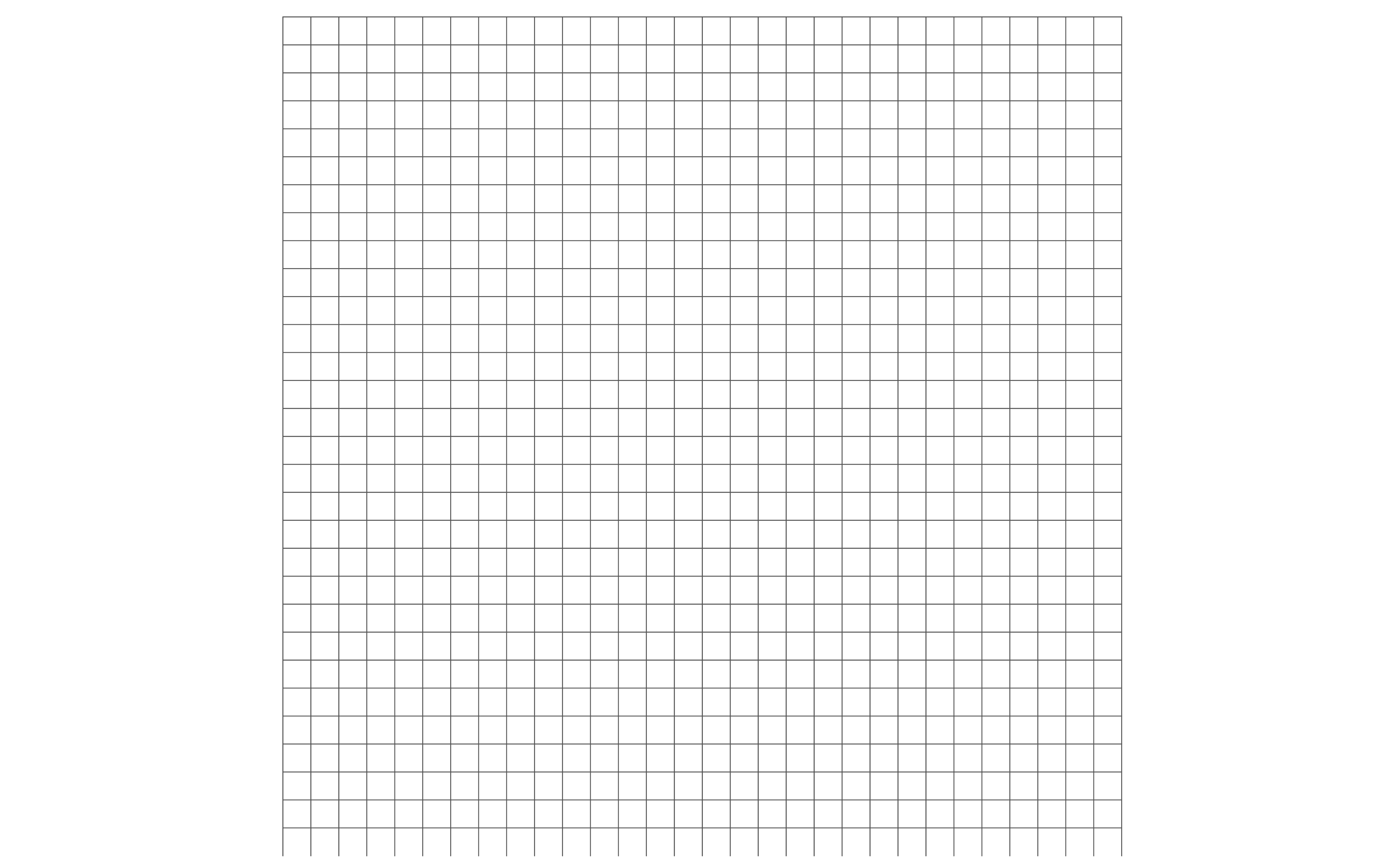
I wanted to start with a grid so that I can easily see what my canvas dimensions would actually look like. Here, I ran into my first challenge: do I actually know how to draw a grid? Of course I can draw one on paper, but how do I code one?
Thankfully it was pretty straight forward once I gave it a bit of thought – I just needed the number of vertical lines (grid_x_size), the number of horizontal lines (grid_y_size), and the space between them all (grid_square_size). I coded this by looping through grid_x_size and drawing a line at each tick, which were spaced by grid_square_size, then doing the same with grid_y_size.
Here's our code for drawing the grid:
import math
import turtle as t

# DEFINE THE DESIRED GRID

grid_x_size = 30
grid_y_size = 30
grid_square_size = 40

grid_width = grid_x_size * grid_square_size
grid_width_half = grid_width / 2
grid_height = grid_y_size * grid_square_size
grid_height_half = grid_height / 2

# DRAW A GRID

def draw_grid(grid_color):
        t.pencolor(grid_color)

        for qx in range(grid_x_size + 1):
            tick_x = (qx - (grid_x_size / 2)) * grid_square_size
            t.penup()
            t.goto(-grid_width_half, tick_x)
            t.pendown()
            t.goto(grid_width_half, tick_x)

        for qy in range(grid_y_size + 1):
            tick_y = (qy - (grid_y_size / 2)) * grid_square_size
            t.penup()
            t.goto(tick_y, -grid_height_half)
            t.pendown()
            t.goto(tick_y, grid_height_half)
And here's the resulting 30x30 grid:
The flow field
Now that I have my canvas gridded out, I want to visualize the "flow field" that my canvas will have. Visually speaking, this is the "movement" of the canvas. Functionally, this is basically where any given point on our canvas (an X/Y coordinate) has an angle that will determine where our generated lines will "travel".
First we can set up the code that will take an angle function and then draw out a grid of points, each with a small line that is oriented to that angle:
def draw_dots_and_angled_ticks(angle_func: callable):
        t.pencolor("black")
        t.penup()

        radius = grid_square_size / 2

        for k in range(grid_x_size + 1):
            tick_x = (k - (grid_x_size / 2)) * grid_square_size

            for p in range(grid_y_size + 1):
                tick_y = (p - (grid_y_size / 2)) * grid_square_size

                # DRAW THE DOT
                t.goto(tick_x, tick_y)
                t.dot()

                # CALCULATE THE ANGLE FOR THE CURRENT TICK
                current_coord = t.position()
                angle = angle_func(current_coordinate=current_coord) # THIS IS WHERE WE USE AN ANGLE FUNCTION (SEE NEXT CODE BLOCK)
                angle_x = radius * math.cos(angle)
                angle_y = radius * math.sin(angle)

                # DRAW THE TICK LINE
                t.pendown()
                t.goto(tick_x + angle_x, tick_y + angle_y)
                t.penup()
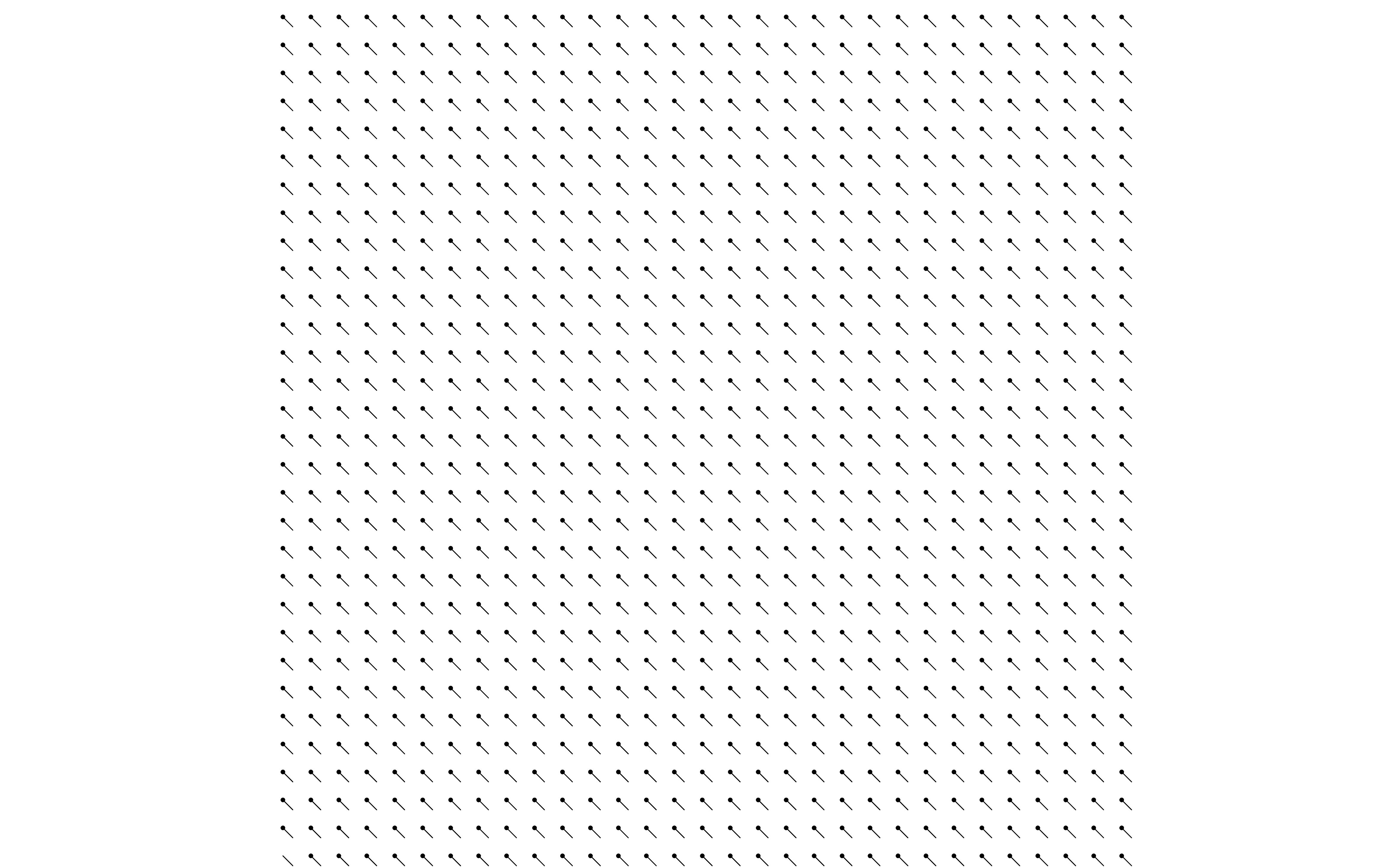
Here's an example of a basic, uniform angle function that we can use as an input to the function above:
def basic_angle_func_() -> float:
    return math.pi * 1.75
We didn't even use point coordinates as an input – all angles will be the same:
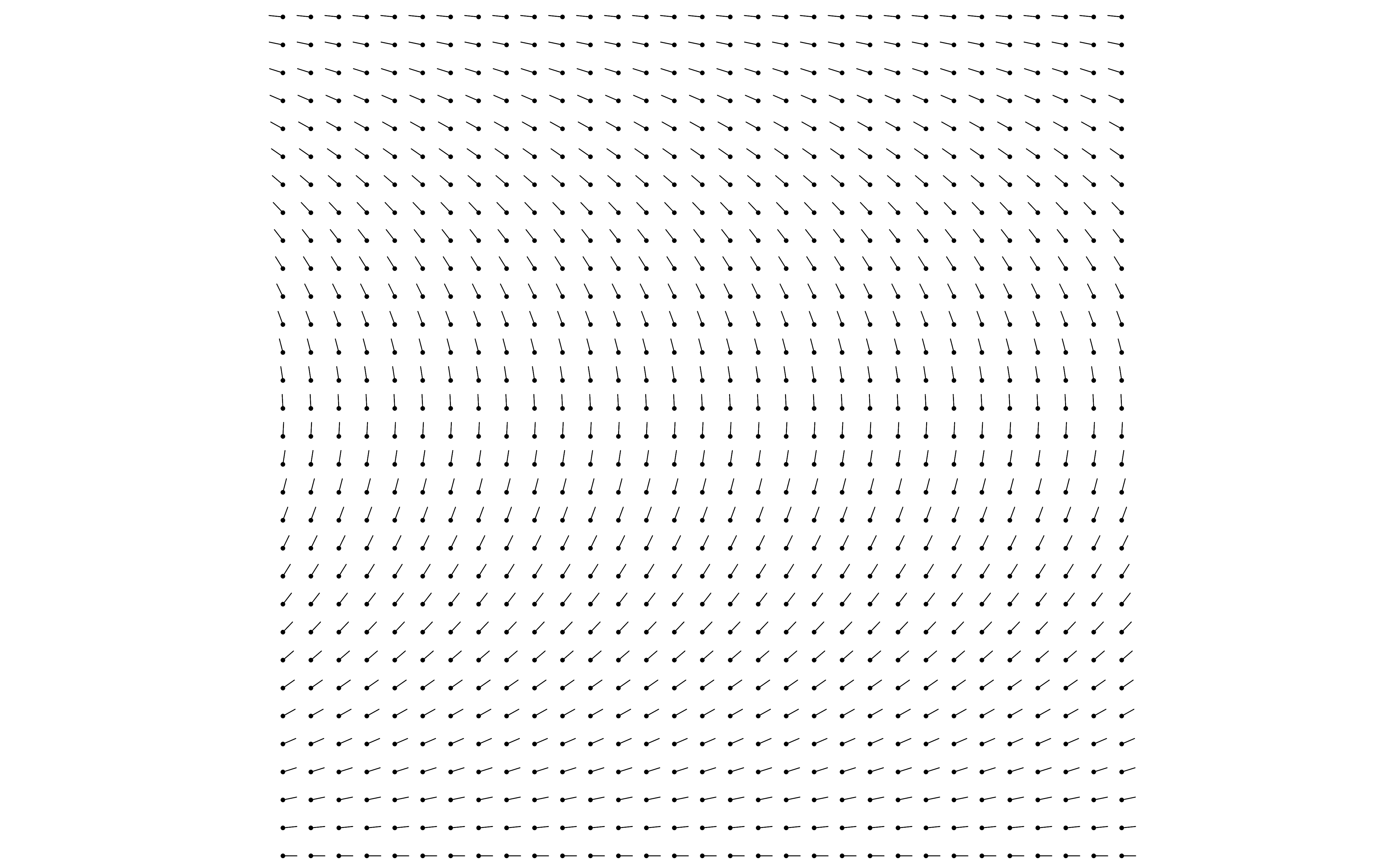
Now, when we do use the point coordinates as an input, we can get a more "flowy" flow field:
def better_angle_func(current_coordinate: Iterable) -> float:
    p = (current_coordinate[1] / grid_square_size) + grid_y_size / 2
    return math.pi * (p / (grid_y_size + 1))
Here's what that would look like:
Adding lines
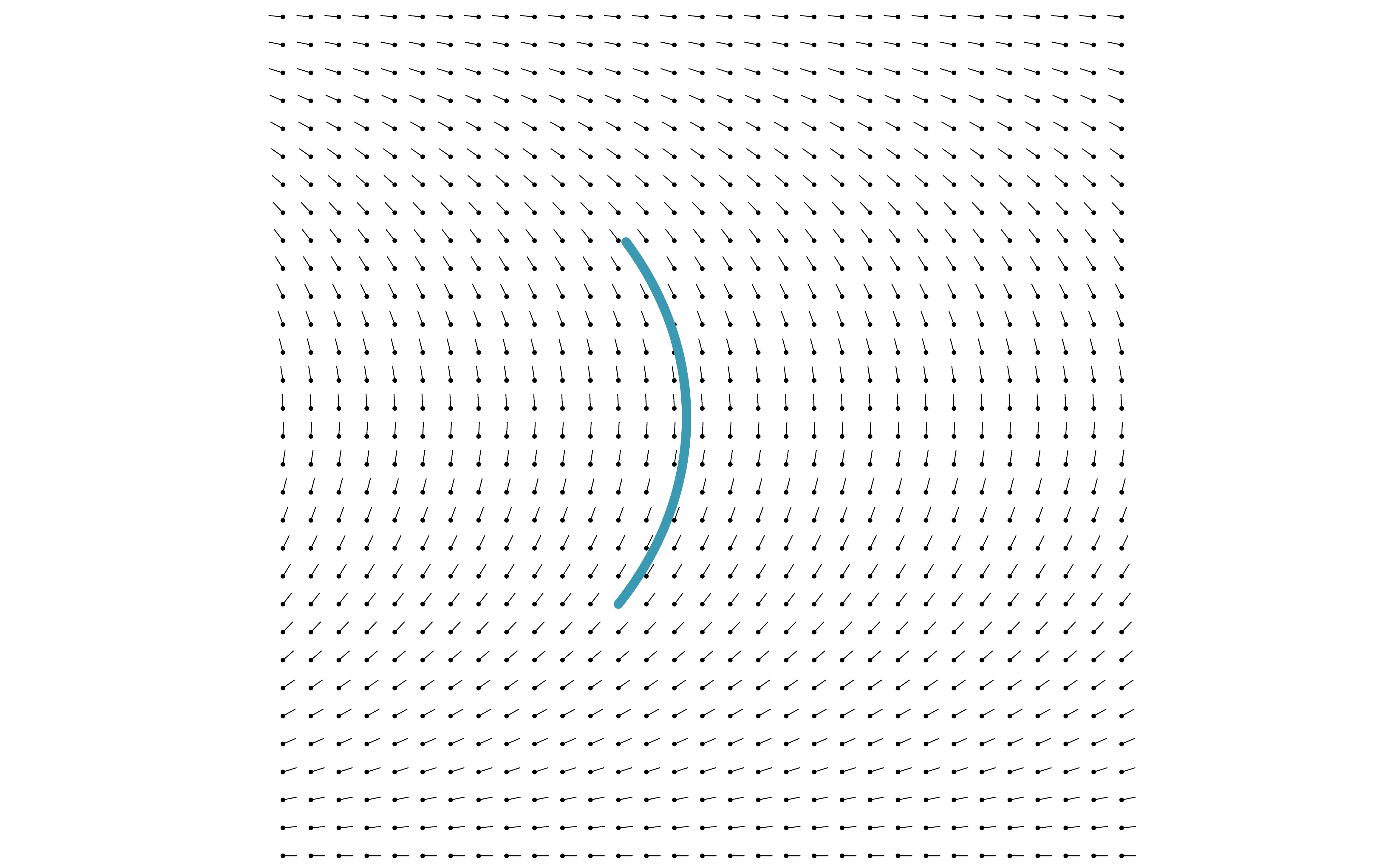
Now we want to start drawing on our canvas. Let's start by just generating a single line at a random starting point and have it drawn in around 30 steps. This means that starting at a given point, we calculate the angle at that point and then draw one "step" in the direction of that angle. Now we're at a new point, so we get the angle for our new coordinates and then draw another step in the direction of that angle.
Here's the code we can use for drawing lines on our canvas:
import random

def draw_lines(
        angle_func: callable,
        pen_color_func: callable,
        num_of_lines: int = 100,
        step_size: int = 20,
        random_thickness_min_max: list = [1, 10],
        random_steps_min_max: list = [10, 20],
    ):
        for l in range(num_of_lines):
            steps = random.randint(random_steps_min_max[0], random_steps_min_max[1])
            rand_start_x = random.randint(
                -(grid_x_size / 2), (grid_x_size / 2)
            )
            rand_start_y = random.randint(
                -(grid_y_size / 2), (grid_y_size / 2)
            )
            rand_thick = random.randint(
                random_thickness_min_max[0], random_thickness_min_max[1]
            )

            t.pensize(rand_thick)
            t.penup()

            starting_point = {"x": rand_start_x, "y": rand_start_y}
            starting_coords = {
                "x": starting_point["x"] * grid_square_size,
                "y": starting_point["y"] * grid_square_size,
            }
            current_coord = list(starting_coords.values())

            t.goto(current_coord)
            t.pendown()

            for j in range(steps):
                current_x, current_y = t.position()

                # CALCULATE THE ANGLE FOR THE CURRENT TICK

                if pen_color_func:
                    t.pencolor(pen_color_func(line_iter=l, step_iter=j, step_total=steps))
                else:
                    t.pencolor(palette.pick_random_palette_color())

                p = (current_y / grid_square_size) + grid_y_size / 2

                angle = angle_func(current_coordinate=t.position())

                angle_x = step_size * math.cos(angle)
                angle_y = step_size * math.sin(angle)

                # DRAW THE TICK LINE

                t.goto(current_x + angle_x, current_y + angle_y)
Okay, now let's loop through 30 steps:
Exciting!
Using color palettes
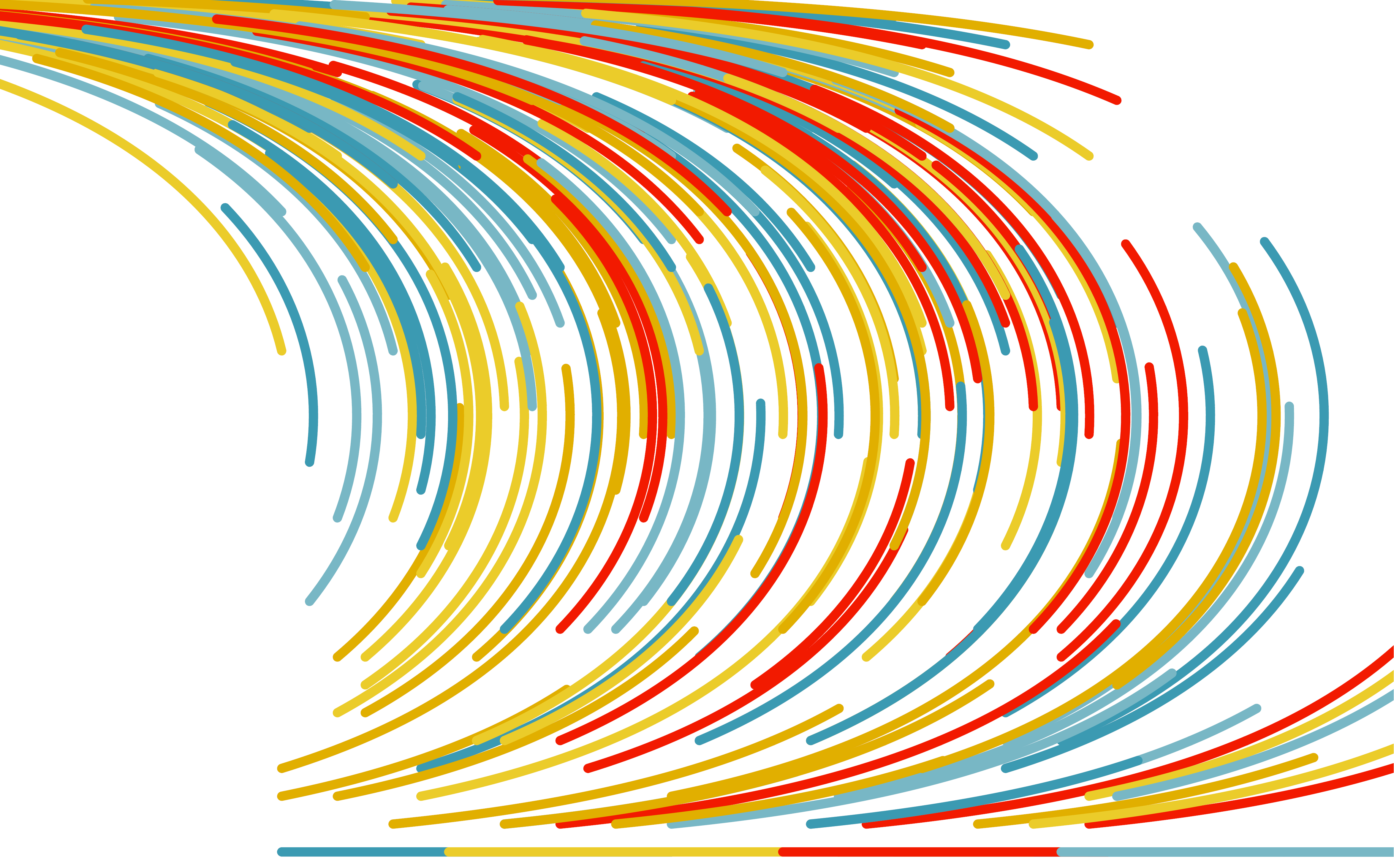
Let's ditch our grid background and draw more lines with some fun colors added in. I'm going to use a color palette from the incredible Wes Anderson pallete R library created by Karthik Ram.
Here's an example where we generate 200 lines where each one uses a random color from the color palette of the movie The Life Aquatic with Steve Zissou using the same angle function we used above:
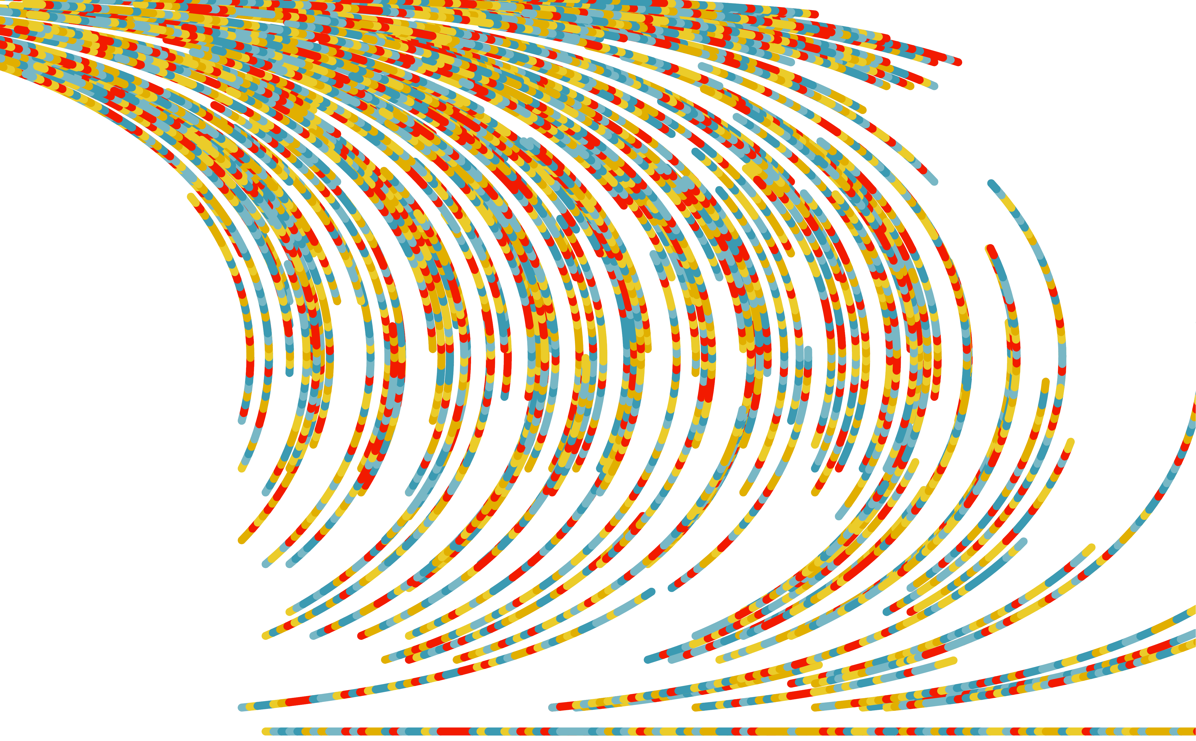
And here's one where we randlomly choose a color from our palette for each step of a line:
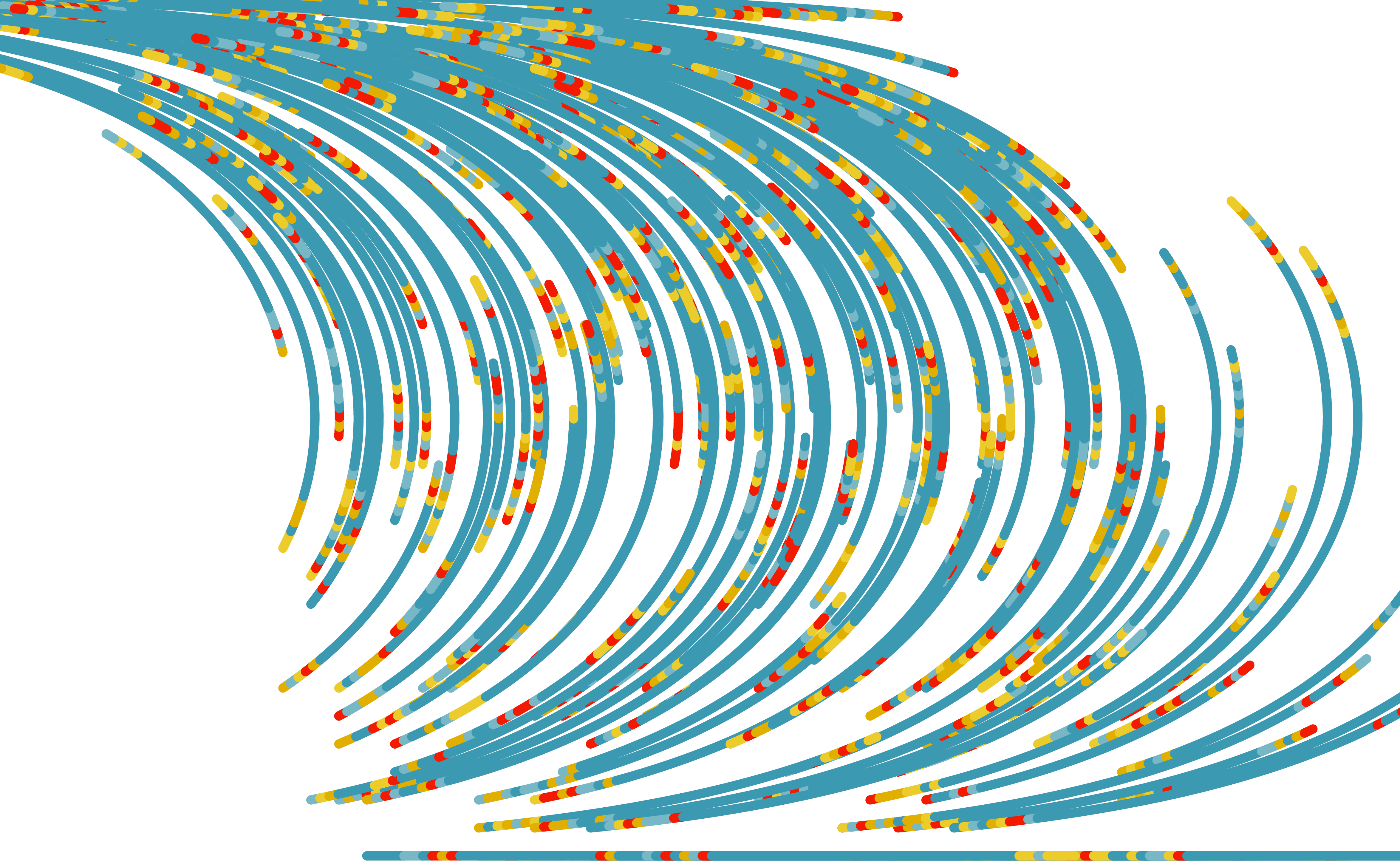
We can make that a little less hodge-podgey by using a color function that uses the primary color for the middle 70% of the line and then a random color from our palette for the beginning 15% and ending 15%:
def somewhat_random_colors(step_iter: int, step_total: int) -> str:
    r = step_iter / step_total
    if r > 0.15 and r < 0.85:
        return palette.palette[0]
    else:
        return palette.pick_random_palette_color()
That would result in this slightly-less-offensive creation:
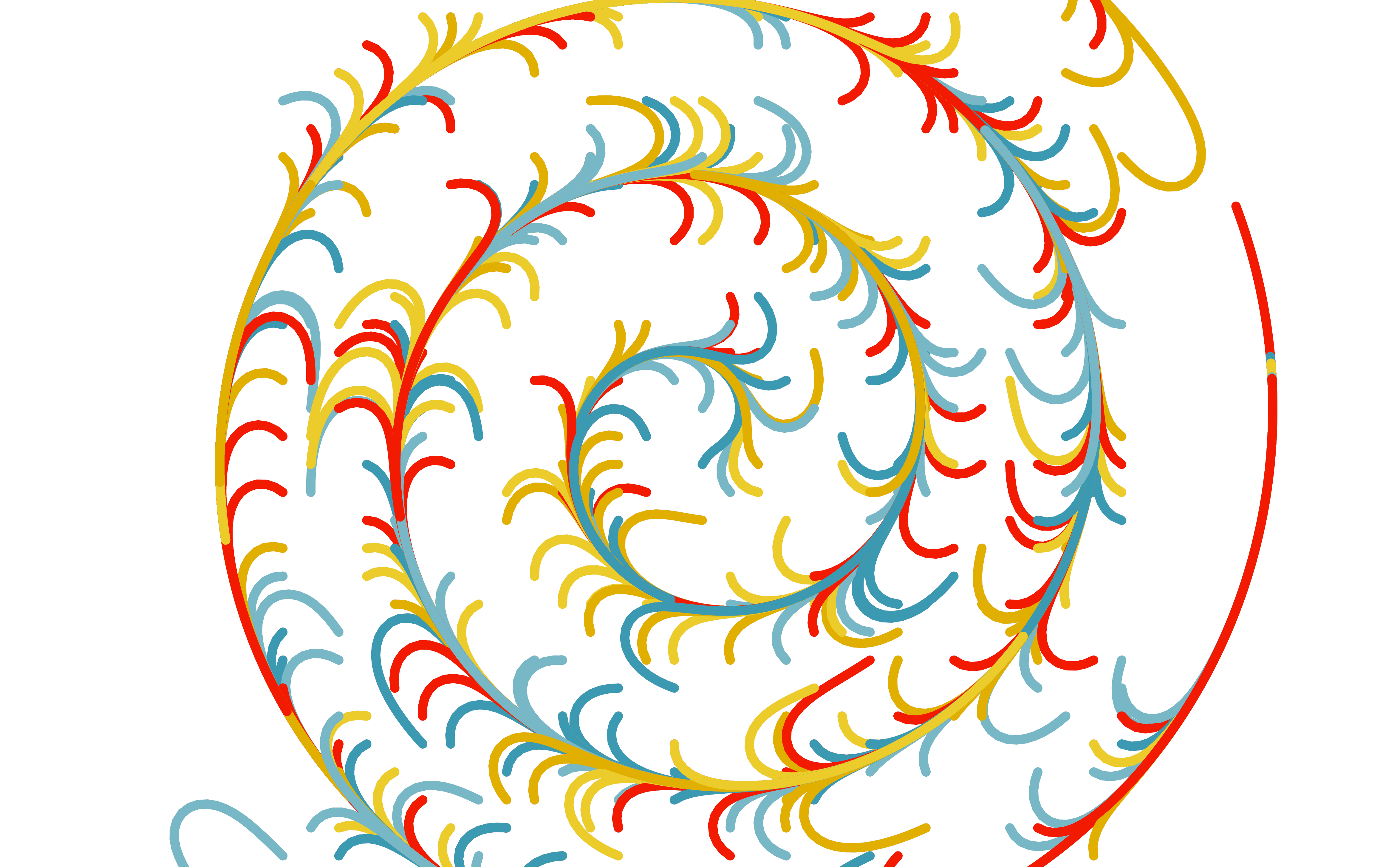
We can switch up our angle function to get a new pattern:
def whirlpool_effect(current_coordinate: Iterable) -> float:
    return math.dist(current_coordinate, (0, 0)) / grid_square_size
Here's our whirlpool effect:
Adding noise
One of the most interesting things that I learned from Tyler's article was about how one can use "noise" generation to get some really beautiful variation in our flow field. Perlin noise was created by Ken Perlin in the 1980's to give CGI graphics more realistic textures. I used the wonderful noise Python library written by Casey Duncan.
Here's an angle function we can use to generate Perlin noise:
def perlin_noise(current_coordinate: Iterable) -> float:
    ns = (
        noise.pnoise2(x=current_coordinate[0] * 0.005, y=current_coordinate[1] * 0.005)
        * math.pi
    )
    return (math.pi * ns) / grid_square_size
Here's an example of drawing 600 thin lines using the function shown above:
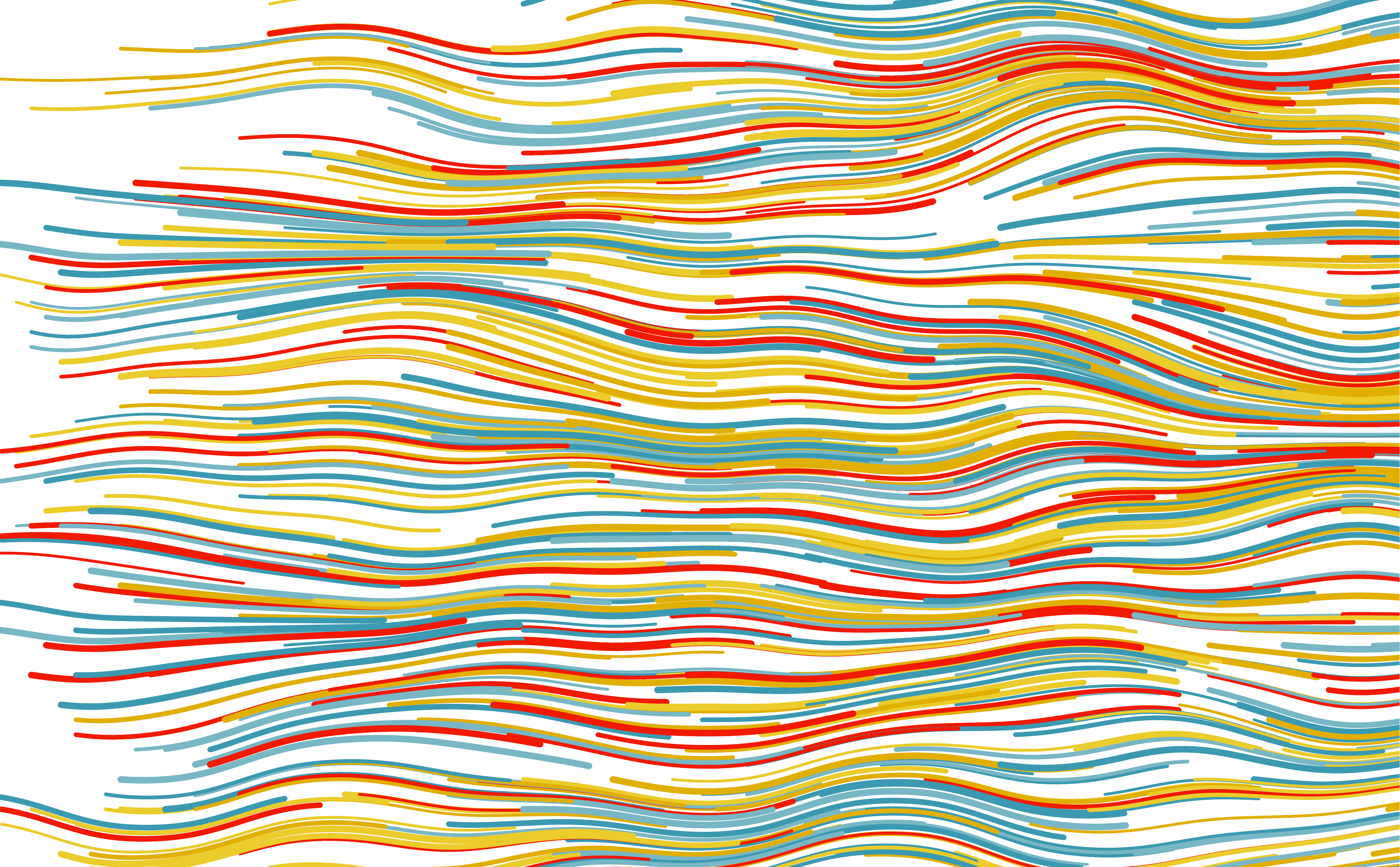
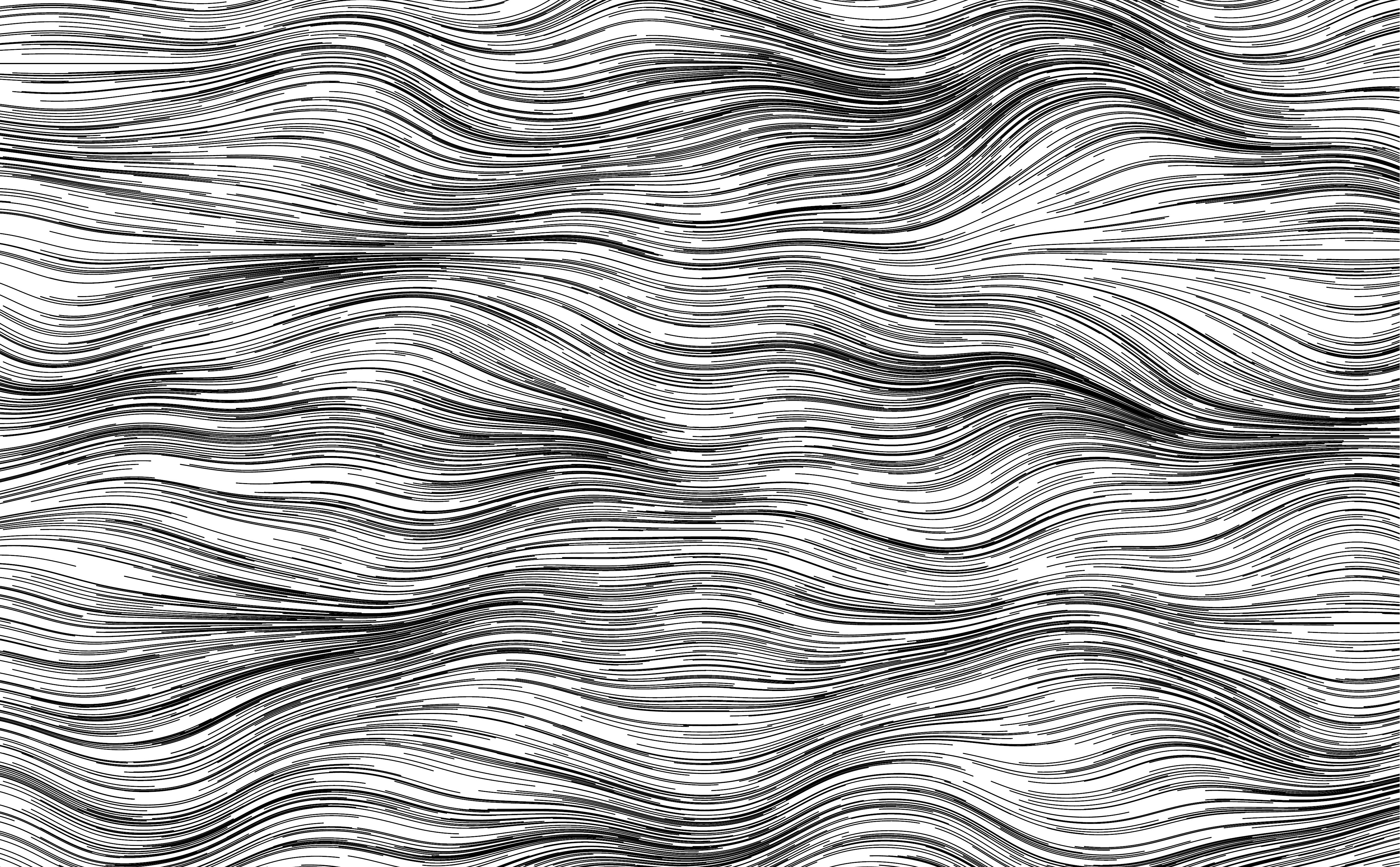
As you can see, we can get some really interesting variation in our flow field using Perlin noise. When we make our lines thinner, longer, and more numerous, and make our grid much bigger, we can get some really beautiful movement:
I'm smarting!
Takeaways
I'm absolutely thrilled with how this all turned out! This project was a chance for me to do and learn about things that I'd never even thought about before, including drawing with code, thinking mathematically and programatically about visual design, and randomness/pseudo-randomness in art.
I feel like a have a new appreciation for the effort and considerable knowledge artists have to create really beautiful and rich art pieces.
Acknowledgements
- Tyler Hobbs (🐙 @thobbs | tylerxhobbs.com) for the inspiration to take on this little project, as well as for writing a fantastic article on the math and ideas behind an art project like this one.
- Casey Duncan (🐙 @caseman) for the
noisePython library. - Karthik Ram (🐙 @karthik) for the Wes Anderson color palettes
- Creators and maintainers of
turtle,tkinter, Python, and VSCode!
